
Hexagonal heatmaps and clever clustering
What it is all about
A wise man once said “Premature optimization is the root of all evil….”. A quote by Donald Knuth with an often forgotten continuation: “…yet we should not pass up our opportunities in that critical 3% [of inefficiencies]”. So what if we could improve core calculations by an order of magnitude and make them blazing fast with one simple elegant trick?
Here at Disy we process, filter and display data using our platform Cadenza. This platform offers many tools for visualization of data and for this blog post we want to focus on a subset of those possibilities, namely:
- Spatial point data on a projected map
- Heatmaps
- Clustering
For some parts of this article I will assume some existing basic knowledge of mathematics and data visualization methods in maps, yet I will try my best to give comprehensive explanations.
Big data
Excuse the buzzword, but it fits the problem we want to solve: Imagine we have a dataset with many points, like crimes in Chicago, ranging from small thefts to big burglaries or domestic violence. The total dataset consists of over 6 million entries and was started in the year 2001! Each point is the reported location of the incidient and clearly we want to find out which regions we should avoid on our next holiday trip.
To clean the dataset from rows that lack spatial information use this quick and dirty command line tool which removes the row if the last three columns (longitude, latitude and point) are empty:
sed -i '/.*,,,/d' DownloadedCrimesFile.csv
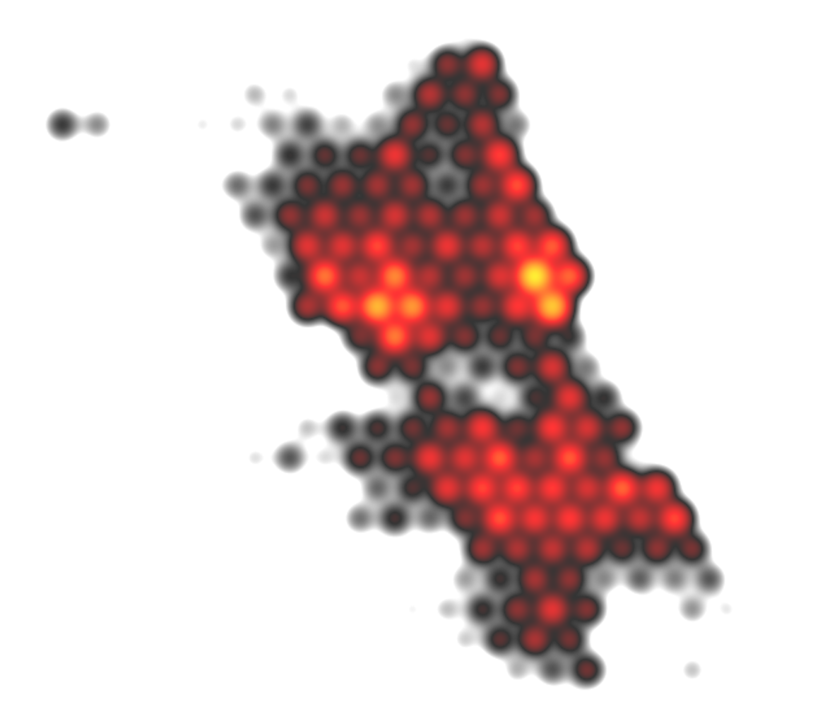
A simple and elegant way to gain insight is to generate a heatmap of the available data. We will use a kernel density approximation for this use case, which you can imagine like a bell-shaped curve which is being put over each individual point and then all of these curves’ values are summed up.
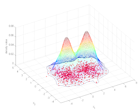
A first implementation could just directly use all invididual points and start its calculations, unfortunately this would not scale well at all. Depending on the result image’s resolution and the heatmap radius it can already take about 10 minutes to render a single heatmap for 6 million points without any special optimizations. That’s not a particularly fast.
What now? Looking a little bit closer at our heatmap, we notice it is used to give a visually smooth and continuous view on the data. So couldn’t we just round something? Maybe round down location data to the nearest integer and be happy about it? No we can’t! We need to support multiple coordinate systems and spatial reference systems, be robust to panning and zooming and other transformations that could happen on the data. We need those floating point values and need to stay in world coordinates instead of doing calculations on the image scale.
If rounding to integers didn’t work out, can you imagine the next step a computer scientist would take to get the upper hand? Binning the coordinates into a grid of squares. It is scalable by adjusting the size according to the order of magnitude of the location values and can be indexed easily and fast via a row and a column.
// properly handle negative x-values!
double index = (long) x - (x < 0. && x != (long) x) ? 1. : 0.;
This approach is very common and definitely the easier way to go, but it inherits one geometric inelegance one should not disregard. Have a look at the following image:
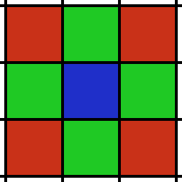
Our blue grid cell has 8 neighbors cells that could contain points which were originally pretty close to each other. But the center of the red neighbors is sqrt(2) times further away from the blue cell’s center than the green neighbors are. This distortion is fundamental to rectangular grids. It’s not awful, but it’s inelegant.
A natural solution
What if we used something nature came up with much earlier than mankind? Honeycombs: A hexagonal structure that tiles our two dimensional plane with minimal boundary and additionally treats all of its neighbors equally.

Sounds too good to be true? Almost, one caveat though is the calculations required to get the honeycomb’s index for some given world coordinate. For a lot of great information and discussions about various hexagon related topics, visit redblobgames, a great resource not only for game developers. Have a look at a “branchless” solution published by Charles Chambers, one that your (JIT) compiler will thank you for.
// normalize grid cells
double relativeX = x / (Math.sqrt(3.) * honeycombRadius);
double relativeY = y / honeycombRadius;
// calculate row and column (columns are axial too and NOT offset)
double temp = Math.floor(relativeX + relativeY);
double honeyRow = Math.floor((Math.floor(relativeY - relativeX) + temp) / 3.);
double honeyColumn = Math.floor((Math.floor(2. * relativeX + 1.) + temp) / 3.);
Looking at that code one might wonder how it works. Because there was no explanation provided at redblobgames I will present one here.
The sqrt(3)is derived from the inner angle: sin(60°). But the rest?
Here’s how you can see why the calculation for honeyRow works the way it does:
A regular hexagonal grid

is normalized (so we are now in relativeX/relativeY coordinate space)

Then we overlay an imaginary rectangle grid, here visualized in dark green

There are 3 (notice, that’s the 3 we divide by) different patterns. For each row the pattern is the same and they repeat depending on the modulus of y (assuming the world y-axis points upwards here). With a simplification of the formula to calculate the honey row, we can then see why it works:
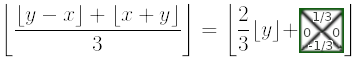
The “height” of a row is the distance taken to get from one point to the equivalent point one row higher and equal to 3/2 in the relative coordinate space. That’s the reason for the multiplication by 2/3: We transform from a world-unit to a row-index-unit.
- It will round down for blue when in the lower triangle (
y%3=0). Number example:2/3*floor(9.4)=6(row 6, rounds down to row 5 if in lower triangle). - It will round up for red when in the upper triangle (
y%3=1). Number example:2/3*floor(10.1)=6+2/3(row 6, rounds up to 7 if in upper triangle). - It will be unchanged for green (
y%3=2). Number example:2/3*floor(11.4)=7+1/3(always row 7).
The calculation of the column can be done analogously and is left as an exercise for the reader (ha, noticed I’m a mathematician?). It helps to think of the input values z as z=floor(z)+remainder(z) with a remainder in [0,1).
Conclusion
Remember the 10 minutes for 6 million points? We are now at 2.5 seconds and there is almost no visual information lost as points are quite dense anyways (of course this depends on the zoom level). Using the techniques described, we could achieve an improvement for heatmap rendering in a range from 10 to 250 times faster calculations compared to the regular calculation with almost no visual difference! These promising results could then be extended to the calculations of clusters which highly profit from neighbors with equal distances from eachother. Further optimizations are possible: Why not let the database do these gridifications and reduce the load on the server(‘s memory)?
It’s fascinating how the ancient idea of a regular grid can improve performance and offer many new ways to solve problems from various different domains. Additionally the elegant symmetry of a hexagonal grid can further be used to handle problems that require big grid cells and yet do not want to suffer from visual distortions.
A lot of fine tuning and thorough testing is involved to balance the trade-off between speed and quality, but that’s a struggle that might be familar to some of you.
Hey, that second frame seems to be a nice visualization for itself, maybe also usuable with discrete colors, like a classification? I think I got a new idea…
The title image is by delfi de la Rua on Unsplash; The kernel density visualization plot and the honeycomb image are from Wikipedia; All other images were created by the author using Gimp, Imagemagick and of course: Cadenza.
Share via


