BigGIS database comparison
Master thesis: Comparing database performance with spatial data
I started my master thesis at Disy in the middle of September. I spent the first weeks getting accustomed to this new experience as well as learning my way around the different database systems I would be working with. After the first few weeks I was able to think about the detailed content of my thesis and what the main steps would be. In this first blog post I want present a little insight on exactly that.
Objective
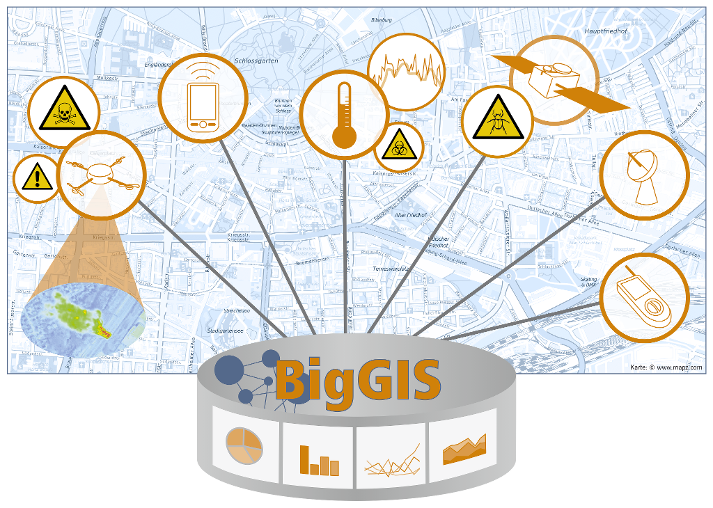
The thesis covers a comparison of different database systems regarding their handling of big spatial data. The thesis is part of a research project called BigGIS. Together with my tutors at Disy we quickly figured out which database systems we wanted to compare in the form of a benchmark. We chose PostgreSQL 9.6, Oracle 12c and EXASolution 5.0. The next question was what should be tested for and with what kind of data? It was decided that the execution time of a series of queries in each system should be compared. The hardware utilization does not play a large role because the EXASol system works completely different than the other two from a hardware perspective. In addition to the runtime comparison, a number of soft factors (e.g. the extent of the functionalities from each system) will be considered. Regarding the data, the benchmark will be tested with custom-built synthetic data as well as with in-house data from Disy.
Creating synthetic data therefore was the first task before the benchmarking could begin.
What’s done so far?
So far several important parts have been completed, most of them had the purpose to prepare the benchmark, additionally some theoretical points of the thesis were also done. First I prepared a lot of theoretical information, including chapters about big data in general and spatial big data specifically. Also there is a large part about the different database systems used as well as an overview about database systems at large.
Going back to the more practical parts which have been done so far, there are mainly two things. - The correct installation of the setup which included the installation of the three test systems on virtual machines as well as establishing a connection from my OS to them. - Creating synthetic data and migrate it to all three database systems
Creating synthetic data
For testing I had to create a synthetic spatial dataset. I started by using R and was easily able to create point and line geometries.
pp <- runifpoint(100,win=owin(c(0,10),c(0,10)))

X <- psp(
        runif(100, min = 0, max = 10),
        runif(100, min = 0, max = 10),
        runif(100, min = 0, max = 10),
        runif(100, min = 0, max = 10),
        window=owin(c(0,10),c(0,10))
        )
However, the import proved to be cumbersome, especially with more complex geometric objects. Therefore I changed from using R to PL/SQL which can create geometric data directly in Oracle. The data then just has to be exported to the other two systems. The polygons I created describe a circle, the creator can simply change the number of points used to create one polygon. With that one can change the complexity of the tested objects. To create a simple polygon with 8 points one would use the following function:
create or replace function generate_polygon(
    ...
    v_cur_radian number := 0;
    ...
    begin
        while v_cur_radian < asin(1)*4 loop
        ...
        v_cur_radian := v_cur_radian + 0.7853;
        end loop;
        ...
    end;
/
In a second part this function then is used to fill a table of the dataset:
DECLARE
   i integer:=1;

BEGIN
   while i < 2501 loop
     dbms_output.put_line(i);
    insert into simplepolygons (id,geom)
      Select
        i,
        generate_polygon(
            p_min_radius =>DBMS_RANDOM.value(low => 500, high => 1000),
            p_lon =>DBMS_RANDOM.value(low => -180, high => 180),
            p_lat => DBMS_RANDOM.value(low => -90, high => 90)) from dual;
        i:=i+1;
   end loop;
END;
/
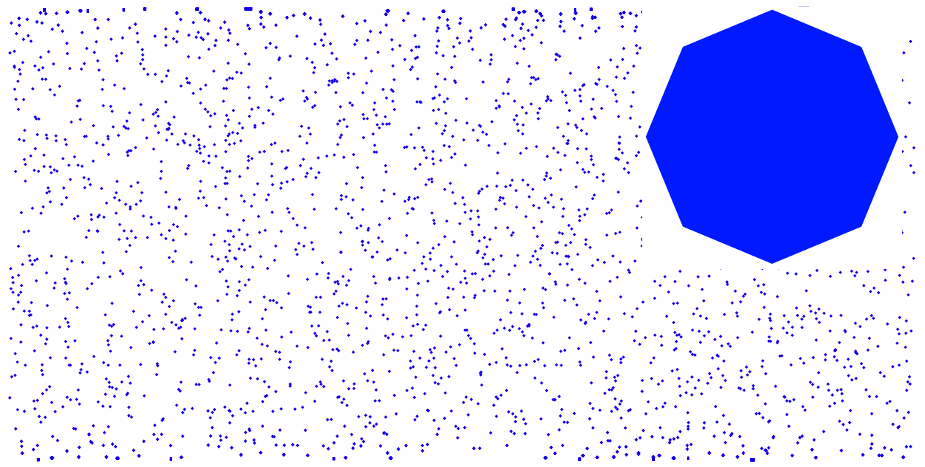
This will create 2500 entries, the polygons will have a constant complexity, but vary in size. They are also randomly distributed inside a predefined area.
In the following screenshot you can get a small impression of the distribution and how one polygon looks like.
For more information on the topic, see the following presentation Presentation
Next steps
The next steps now are to finish the data import for each database system and to classify the database queries into fitting categories. First of all, the queries will be separated into simple and complex ones. They then will be distributed further into groups which handle data in a similar way (e.g. group all relate funtions from Oracle into one category). After the queries have been classified, they will be run on each system to measure the execution time. Comparing the result in combination with the soft factors will allow to draw conclusions on the strengths and weaknesses of each database system. The hope is that the results make it possible to give recommendations which system might be the best for different user groups (e.g. private users, companies or academic purposes).
The last big chapter will focus on new developments in the scene regarding the problematic handling of three dimensional data and big spatial temporal data.
The title image BigGIS was published by Forschungszentrum Informatik FZI.
Share via


